Latin Hypercube Sampling
What is LHS?
Latin hypercube sampling aims to bring the best of both worlds: the unbiased random sampling of monte carlo simulation; and the even coverage of a grid search over the decision space. It does this by ensuring values for all variables are as uncorrelated and widely varying as possible (over the range of permitted values).
Why do I need one?
The background to this is that I have been working on improving the convergence of an optimisation package that uses genetic algorithms. Having a good distribution of “genes”, or decisions within the initial population is key to allowing a GA to effectively explore the decision space. The ga() function within the GA package in R allows for a suggestions argument, which takes a matrix of decision values and places them within the starting population. Initially I wrote one function to create evenly spaced sequences for every decision between the lower and upper bound of allowable values, from which I enumerated all possible combinations using expand.grid(). I then wrote another function to take a model object and a user-defined population size and automatically work out the nearest population count that allowed for even sampling over the model’s decision bounds.
For models with large numbers of decisions the potential number of combinations is enormous. This is true even if you only select the upper and lower bound per decision. Already with 30 independent decisions with two possible values the number of combinations is 2^30 = 10,737,41,824, 10 times more than the number of stars in the average galaxy. Combinatorial algorithms are the worst type for growth in complexity (\(O(n!)\)). I needed a way of randomly sampling from the decisions but in a way that ensured the starting population had lots of diversity. This is the exact use case for LHS.
Practical examples
Let’s assume we have three decisions, where:
- decision a can be between 1 and 3,
- decision b can be TRUE or FALSE, and
- decision c can be red, green, blue or black
There are \(3 * 2 * 4 = 24\) possible unique combinations of these decisions (if a can only take on integer values). An individual in the starting population of a genetic algorithm would be of the form, 1_TRUE_red, for instance.
Let’s assume we would like only 12 individuals from the 24 potential unique combinations, but we still want good representation of all/most possible decisions. Using the lhs library from R, we first create 12 random uniform distributions between 0 and 1 for each of the three decisions, a, b and c.
##             a          b          c
## 1  0.33294610 0.10451561 0.74941994
## 2  0.08062376 0.32965333 0.46038286
## 3  0.58735423 0.88374202 0.36045797
## 4  0.94940245 0.17358330 0.80232318
## 5  0.36656711 0.58122048 0.25851211
## 6  0.54630103 0.97777021 0.88724164
## 7  0.86868358 0.69483831 0.92874699
## 8  0.69615823 0.42490342 0.02729945
## 9  0.47484290 0.76646097 0.24412198
## 10 0.13634272 0.03092663 0.55401471
## 11 0.75789241 0.37229270 0.13919799
## 12 0.21069690 0.63134148 0.59831409
Next we map the 0-1 distributions onto the real distributions of a, b and c. For instance, c has four possible values so the distribution should be 1-4. We also convert the values to factors in order to label them properly.
# Random choices for each decision with distributions based on a, b and c
choices <- map2(sample, all_decisions,
                ~cut(.x, length(.y), labels = as.character(.y))) %>%
  bind_rows()

choices
## # A tibble: 12 × 3
##    a     b     c
##    <fct> <fct> <fct>
##  1 1     TRUE  black
##  2 1     TRUE  green
##  3 2     FALSE green
##  4 3     TRUE  black
##  5 1     FALSE green
##  6 2     FALSE black
##  7 3     FALSE black
##  8 3     TRUE  red
##  9 2     FALSE red
## 10 1     TRUE  blue
## 11 3     TRUE  red
## 12 1     FALSE blue
For convenience we can bring this into a single function like so.
lhs_sample <- function(decisions, n){
  stopifnot(is.list(decisions))
  len_decisions <- length(decisions)
  samples <- lhs::randomLHS(n, len_decisions) %>%
    as.data.frame()
  names(samples) <- names(decisions)
  choices <- purrr::map2(samples, decisions,
                  ~cut(.x, length(.y), labels = as.character(.y)))
  bind_rows(choices)
}

lhs_sample(list(cars = rownames(mtcars), species = unique(iris$Species), letter = LETTERS[24:26]), n = 10)
## # A tibble: 10 × 3
##    cars                species    letter
##    <fct>               <fct>      <fct>
##  1 Volvo 142E          setosa     X
##  2 Merc 280C           versicolor Y
##  3 Datsun 710          setosa     X
##  4 Merc 240D           versicolor X
##  5 Mazda RX4           versicolor Z
##  6 Lincoln Continental setosa     X
##  7 Lotus Europa        virginica  Y
##  8 Honda Civic         virginica  Z
##  9 Pontiac Firebird    virginica  Z
## 10 Merc 450SLC         virginica  Z
Continuous distributions
The above example was for sampling from distributions where allowable values were either factors or whole integers. For continuous numerical distributions we can use the following.
library(tidyr)
a_continuous <- all_decisions[[1]]

choices_continuous <- qunif(sample$a, min = min(a_continuous), max = max(a_continuous))

choices_continuous
##  [1] 1.665892 1.161248 2.174708 2.898805 1.733134 2.092602 2.737367 2.392316
##  [9] 1.949686 1.272685 2.515785 1.421394
Testing coverage
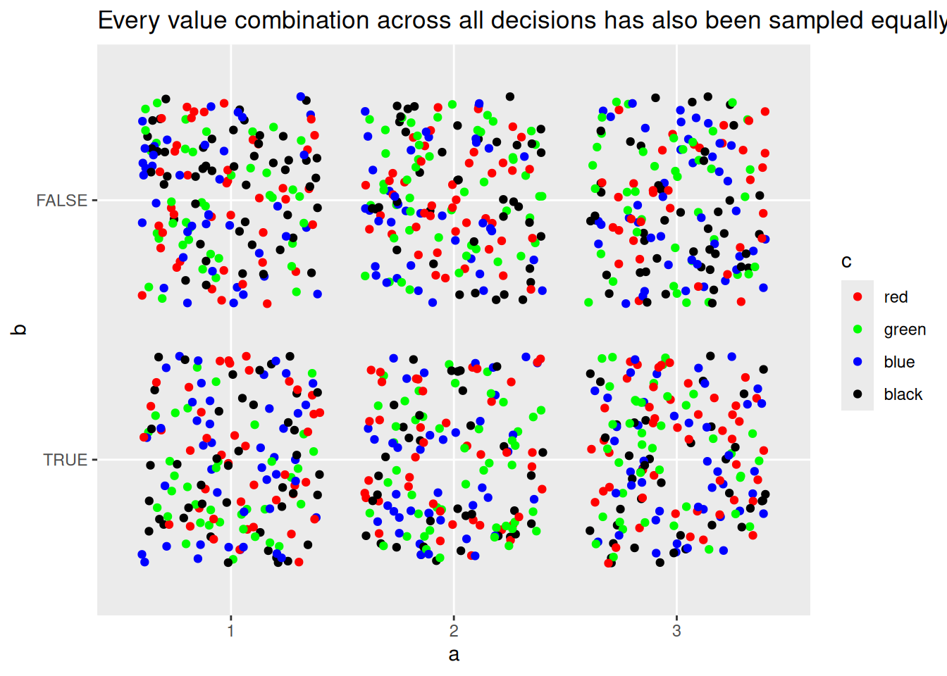
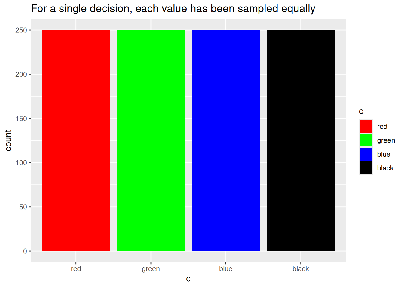
In theory, each sample should be orthogonal, or independent, of each other sample to the greatest possible extent. Another way of putting it is that there should neither be any one value overrepresented or under-represented in the sample set. Let’s test this in practice:
library(ggplot2)
big_sample <- lhs_sample(decisions = list(a = a,b = b,c = c), n = 1000)

ggplot(big_sample, aes(x = c, fill = c)) +
  geom_bar() +
  scale_fill_manual(values = c("red", "green", "blue", "black")) +
  labs(title = "For a single decision, each value has been sampled equally")
ggplot(big_sample, aes(x = a, y = b, colour = c)) +
  geom_jitter() +
  scale_colour_manual(values = c("red", "green", "blue", "black")) +
  labs(title = "Every value combination across all decisions has also been sampled equally")